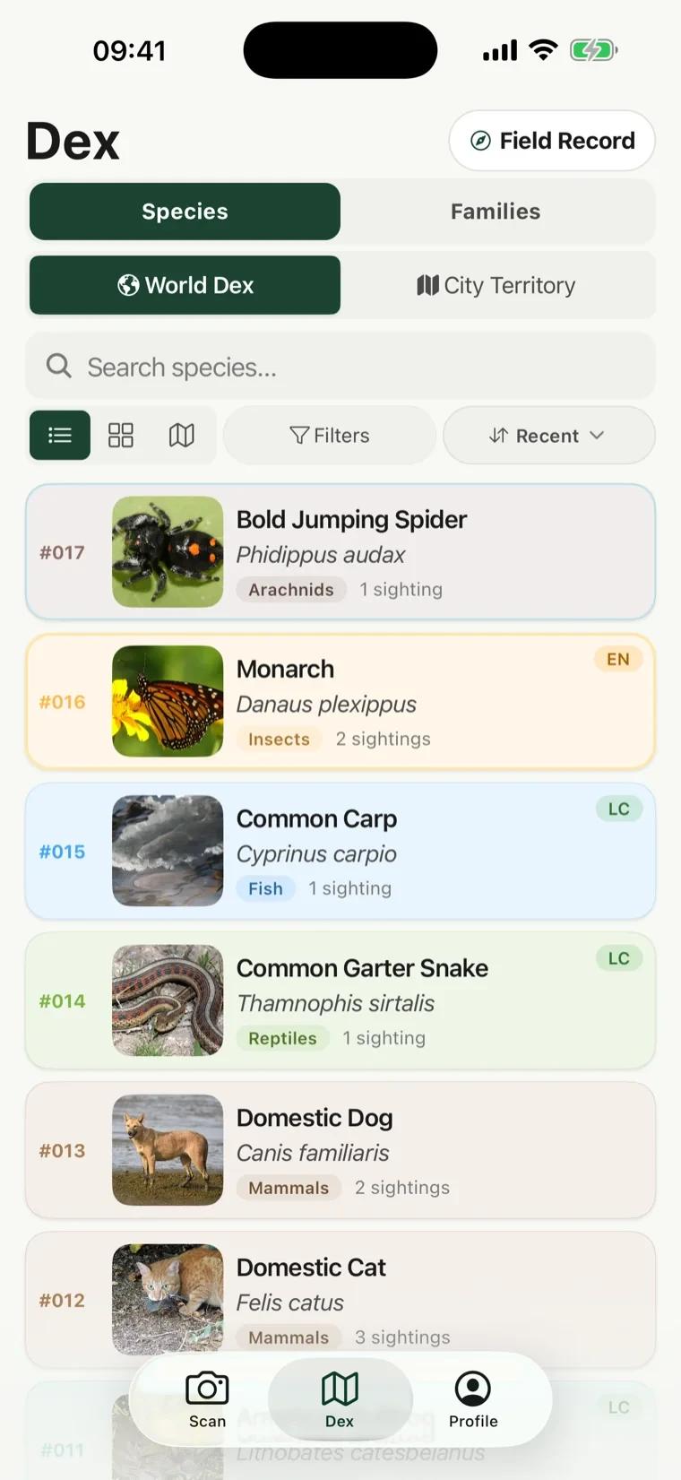
RealDex's original identification model was large, CPU-bound, and less accurate than the app needed.
I trained FieldNet 1, rebuilt the benchmark without data leakage, and shipped a versioned, verified INT8 model pipeline.
39 MB, 5,077 species, and 61.3% top-1 accuracy on the documented holdout, up from a 46.8% BioCLIP baseline.
The first version of RealDex was a packaging problem. BioCLIP is a vision transformer built for scientific-scale biological representation learning, not for a React Native camera app. To get it onto an iPhone and an Android foldable, I converted the graph, replaced operators that mobile runtimes reject, quantized the weights to INT8, and shipped a separate database of species vectors beside it. It worked. That felt like the achievement at the time.
But shipping a model and choosing the right model are two different things. BioCLIP identified species by comparison, not by decision: it turned a photo into a 512-dimensional vector, then measured cosine similarity against one stored prototype per species. The encoder was frozen. It had never been trained to separate the exact 5,077 species RealDex cares about. Confidence was often weak, the transformer graph stayed on the CPU, and the complete first-run AI download reached about 105 MB. So I asked the uncomfortable question: instead of optimizing BioCLIP further, should RealDex replace it?
The answer was yes, and the reasoning was structural. A frozen encoder with nearest-prototype matching leaves accuracy on the table by design, because nothing in the pipeline is ever trained on the actual label space. A trained classifier decides directly. It also maps onto mobile accelerators far better, because a convolutional graph is what phone GPU delegates are built to run. The plan was to keep RealDex's existing YOLO detector as a gate and its cloud verification as a fallback, and to replace only the part in the middle: the thing that names the animal.
Training the model was not the hard part. Three failures were, and each one stayed invisible until it had already done damage:
My first head-to-head comparison favoured BioCLIP, and the comparison was invalid. Some of the images used to build BioCLIP's species prototypes also appeared in the evaluation pool. BioCLIP was being tested on pictures it had effectively already memorized, while my new model was tested cleanly. This was not a bug in the shipped app. It was a bug in the experiment, which is worse, because the experiment is what decisions get made from. I rebuilt every BioCLIP prototype from training images only and ran the comparison again.
The first trained model scored 33.0% top-1 in full precision. Compressed to INT8 for the phone, it fell to roughly 21%. Twelve percentage points disappeared into the conversion. The cause was flat class scores: the model often ranked the right species near the top, but the numerical gaps between candidates were so small that quantization noise reordered them. An accurate model that cannot be compressed is not a mobile model.
The RTX 4080 sat mostly idle while training crawled. The dataset was still on an external USB hard drive, which fed images at about 31 per second. The same working set on an internal SSD fed about 301 per second. At USB speed the remaining epochs were projected to take more than 70 hours. Copying the data took 11.7 minutes. The lesson is unglamorous and worth stating plainly: on a single-GPU training box, the bottleneck is usually not the GPU.
None of this happened cleanly, and the specific shape of each failure is the part worth keeping:
Four phases, each of which had to be right before the next one meant anything:
The source was the iNaturalist 2021 train_mini archive, about 44 GB. A conversion script kept only classes that map to animal categories and discarded plants, fungi, protozoa, and other kingdoms. That left 5,077 animal species: 2,526 insects, 1,486 birds, 313 reptiles, 246 mammals, 183 fish, 170 amphibians, and 153 arachnids. I capped each species at 50 images rather than forcing a perfectly balanced set, and I removed 5 images per species before training started to serve as an untouched final holdout.
FieldNet 1 started from an ImageNet-pretrained MobileNetV4-Conv-L backbone, so it was fine-tuned rather than trained from scratch. Two warm-up epochs trained the new classifier head alone, which protects the pretrained weights while a randomly initialized head finds its footing. The full backbone then unfroze for 38 more epochs at 256x256 input, with RandAugment, Mixup, CutMix, random erasing, label smoothing, stochastic depth, a cosine learning-rate schedule, and an exponential moving average of the weights. The productive run took 7 hours 20 minutes.
To fix the quantization collapse I added six final epochs with Mixup disabled and label smoothing set to zero, training the whole network against hard one-hot targets. This widens the numerical gap between the winning score and its rivals, which is exactly what quantization needs. Training loss fell from about 3.7 to 0.75, but that number proves little on its own — removing softened targets lowers the loss mechanically. The real evidence came after export, when FP16 and INT8 landed within 0.14 points of each other.
FieldNet 1 replaced the retrieval path rather than running beside it, which removed the 10.5 MB prototype database entirely. The app downloads one 39 MB INT8 file after onboarding and verifies its SHA-256 digest before activation, alongside a separately digested label file and geographic prior. The rollout sits behind a Firebase Remote Config flag, so the model could ship dark and be enabled per platform and per version, and every prediction passes a confidence gate before the app is willing to assert a species.
FieldNet 1 INT8 reaches 61.3% top-1 and 81.7% top-5 across 5,077 species, against a leakage-free BioCLIP baseline of 46.8% top-1 and 73.4% top-5. That is a gain of 14.5 percentage points, or roughly 31% relative. INT8 costs only 0.14 points against FP16 while cutting the file to 39 MB. The complete first-run AI download fell from about 105 MB to about 46 MB. Random guessing in this label space would score about 0.02%.
"61% does not sound impressive until you know what it is 61% of. This is 5,077 fine-grained wildlife classes, judged on crops from the same YOLO detector the app actually ships, from a 39 MB file running offline on a phone. I did not feel anything when training finished. I felt it when the comparison table rendered and the fair BioCLIP column was clearly, unambiguously lower."
The charts, artifact manifests, calibration thresholds, and the measurements I am not willing to overstate.
Every number below comes from one protocol. I removed 5 images per species from the dataset before training started, which produced an untouched holdout. I passed those frames through the shipping YOLOv8n detector and kept the 10,918 crops where it found an animal. Every exported model then saw those same 10,918 crops, and I checked each model's class indices against its own matching label file.
The BioCLIP baseline here is the rebuilt one. Its species prototypes were regenerated from training images only, after I found that the original prototypes had absorbed images from the evaluation pool.
10,918 YOLO crops from an untouched holdout
FieldNet 1 gains 14.5 points of top-1 accuracy over the leakage-free BioCLIP baseline. The INT8 model is the one that ships; it costs 0.14 points against FP16 at half the file size.
I have deliberately not published an FP32 accuracy figure for the final model. I evaluated FP16 and INT8, which are the artifacts that could actually ship. Quoting a third number I did not measure would be padding.
The failed run showed a pattern worth understanding, because it only appears after export. The full-precision model was mediocre but functional. Both compressed versions were unusable.
Top-1 accuracy by numeric format
Left: the abandoned first run, where compression destroyed 12 points. Right: after six sharpening epochs, both shipping formats agree within 0.14 points. Same architecture, different training endgame.
The mechanism is straightforward once you see it. Mixup and label smoothing train a model to spread probability deliberately, because soft targets reduce overconfidence and improve generalization. They also compress the distance between the top candidates. INT8 quantization then rounds those already-narrow gaps, and the ranking scrambles.
Six sharpening epochs reversed it. Mixup off, label smoothing at zero, whole network trainable, hard one-hot targets. The model learned to commit. Training loss dropped from roughly 3.7 to 0.75, which I want to explicitly not present as a breakthrough — removing softened targets lowers the loss arithmetically, whether or not the model improved. The result that mattered was that FP16 and INT8 converged.
This is the thesis of the whole project in one figure. Better is up and to the left.
BioCLIP also needs a 10.5 MB prototype database beside its 88 MB encoder, so its real footprint sits further right than plotted. FieldNet 1 INT8 needs a 0.5 MB label file.
Removing retrieval removed a whole asset class. FieldNet 1 carries a geographic prior instead, which is smaller than the prototype database it replaced.
The most expensive mistake in the project had nothing to do with machine learning.
Images per second reaching the GPU
An 11.7-minute file copy converted a projected 70-plus hours of remaining training into 7 hours 20 minutes. The GPU had never been the constraint.
Every one of those failures was recoverable for one reason: the pipeline checkpointed after every epoch. A corrupted archive, case-insensitive globbing that duplicated files, a missing serving signature on export, a Unicode character that crashed a log path, and three libraries fighting over one Python environment — each cost time, none cost the run.
Two of those entries carried more weight than the rest. The head-only warm-up exists because a randomly initialized 5,077-way classifier produces large, badly aimed gradients at first, and letting those reach a pretrained backbone damages features that took a lot of compute to learn. The exponential moving average keeps a smoothed copy of the weights across noisy updates, so the exported model reflects the trend of training rather than wherever the last step happened to land.
5,077 classes retained from iNaturalist 2021 train_mini
The distribution skews heavily toward insects, and that is a real property of the problem rather than a flaw in the data. Insects genuinely dominate animal biodiversity. It does mean the headline accuracy figure is dominated by the hardest and most visually similar classes in the set, which I consider a fair way to be judged.
FieldNet 1 downloads after onboarding and before the camera first opens. Three files arrive as one versioned pack: the INT8 model, its label file, and a geographic prior. Each is verified by SHA-256 digest, and a mismatch causes rejection rather than a load attempt.
The digest check on the label file is not routine hygiene. It is the load-bearing part.
Replacing retrieval with classification introduced a genuine regression, and it needs stating plainly. BioCLIP could compare a crop against newly generated prototypes, so extending it did not require retraining. FieldNet 1 has exactly 5,077 outputs. Shown an animal outside that set, it must still distribute probability among species it knows.
RealDex therefore refuses to assert a species unless three conditions hold together.
Below those thresholds the app presents ranked local candidates and an explicit option to verify with the cloud. Low confidence never silently spends a cloud identification credit.
This is the section where my own first draft overreached, so it is worth being precise about the limits of the evidence.
BioCLIP era, capture to visible result sheet
Individually measured stages account for about 6.2 of the 11.1 seconds. The rest sat in orchestration, image preparation, state changes, and UI work. These are single-run figures from my own instrumentation, not an averaged benchmark.
On a Galaxy Z Fold5, FieldNet 1 classified through the Android GPU delegate in 44, 50, and 67 milliseconds across three runs, averaging 53.7 ms. It identified the test cat correctly as Felis catus at 43% confidence, with a long-tailed weasel and a mountain lion trailing well behind — wrong answers, but wrong within visually related mammals, which is the failure mode you want.
I am not going to multiply 1,600 ms by anything and call it a speedup. The BioCLIP figure came from an iPhone 13 mini on CPU and the FieldNet figure from a Fold5 on GPU: different silicon, different operating system, different delegate. Two numbers measured that differently do not divide into an honest ratio.
I want the attribution here to be accurate rather than flattering in either direction.
I set the product objective and accepted the architecture change. I set the fairness standard that exposed the benchmark leakage, and I decided the leaky comparison could not be published even though it was the one that had already run. I chose to restart the failed run rather than salvage it. I accepted the closed-set trade-off and specified that confidence had to gate assertion. I decided which numbers in this case study were strong enough to publish.
The instrument was AI throughout. Kimi K3 framed the initial architecture brief and training guidelines. The deeper architecture comparison ran through Claude Code as a multi-agent research pass across BioCLIP, BioCLIP 2, MobileNetV4, EfficientNet, MobileCLIP, and DINOv2, where 22 claims survived three-vote adversarial checking. Claude Opus 4.8 then implemented the training, recovery, export, and benchmark pipeline.
FieldNet 1 ships in RealDex on Google Play, enabled through a Firebase Remote Config flag scoped by platform and version so it can be switched off without a release. The iOS build is pending App Store release and uses the same INT8 artifact on CPU. The live in-camera classification path exists in the codebase but stays disabled: its latency is unvalidated, and shipping an unvalidated real-time path into a camera is how you turn a 54-millisecond model into a janky one.
Train the smallest model that can plausibly work, and evaluate it the way it will ship — quantized, on detector crops, against a holdout you removed before you started. Every shortcut I took around that principle cost me more time than the shortcut saved. The benchmark leakage cost a full rebuild of the baseline. The soft-target training cost six extra epochs and a second export cycle. The USB drive nearly cost three days.
BioCLIP proved RealDex could run serious biological vision on a phone. FieldNet 1 proved the first model did not have to be the final architecture.
My leaky benchmark was automated, deterministic, and numerically precise. It was also rigged, and every one of those good properties made it more convincing rather than less. Rigor is not a reporting step you perform at the end. It belongs in the implementation, next to the code that builds the evaluation set, because a benchmark's job is to be capable of telling you that you were wrong.
BioCLIP was the right first decision and the wrong permanent one. It proved a serious biological vision model could run offline on a phone, which was the question that mattered in version one. Replacing it meant discarding work I was proud of, including the vector loaders and the embedding pipeline. The sunk cost was real. It was also irrelevant to the question of what the product should do next.
The quantization collapse was not an export bug. It was a training decision surfacing three steps downstream, because heavy label smoothing and Mixup produce a model whose confidence is deliberately soft — and soft confidence is precisely what INT8 destroys. I could not fix it in the converter. I had to go back and change how the model was trained. If a model has to run in 8 bits on a phone, that constraint has to be present while it learns.
FieldNet 1 moved RealDex in two directions at once. The shipping INT8 model raised fair top-1 accuracy by 14.5 percentage points while cutting the first-run AI download by roughly 56%. It removed the separate embedding database, survived quantization with a 0.14-point loss, and reached the Android GPU delegate that the old transformer could never use. Products usually trade accuracy against size. This one improved both, because the dataset, training recipe, benchmark, export, and mobile integration were treated as one system rather than five stages.
The number I care about is not 61.3%, or 39 MB, or 54 ms. It is the combination. A model that is accurate but too large is a demo. A model that is fast but unreliable is a gimmick. And a model that beats its predecessor on a benchmark it was allowed to cheat on is neither — which is why the most valuable hour of this project was the one I spent proving my own result wrong before I published it.
 Alp Yalay